Expanding on Controls and PID

In the previous lab, we were able to get our mice driving reasonably straight with just proportional control. This week, we'll learn how to correct for persistent steady state error, turn in place, and follow walls.

For this lab, we'll be using the same starter code as Lab 5. Since this lab is an expansion of the previous one, we recommend just modifying your existing code.

Expanding on Proportional Control

Recall our implementation of a proportional (P) controller from last week.

$$ \begin{align}
e(t) = setp&oint(t) - actual(t) \\
u(t) &= K_p e(t) \\
applyPowerLeft(&u_{linear}(t) + u_{angular}(t)) \\
applyPowerRight(&u_{linear}(t) - u_{angular}(t))
\end{align} $$

Proportional control works pretty well for making our mouse drive straight, but you may have encountered a constant offset error when using it to control linear velocity. If we had zero linear velocity error, we'd apply zero power to our motors, which means they'd stop! How might we fix this? What if we kept track of the total error?

$$ u(t) = K_p e(t) + K_i\int_{0}^{t} e(\tau) d\tau $$

This is called a proportional-integral (PI) controller. The integral keeps track of the total error (both positive and negative) since we first started the controller. Even small errors will cause the integral term to eventually grow large enough and get \(u(t)\) to push our mouse back on track.

In order to dampen oscillations and prevent overshoot, we might want to consider the derivative of our error too. This prevents our error from changing too quickly.

$$ u(t) = K_p e(t) + K_i\int_{0}^{t} e(\tau) d\tau + K_d (de(t)/dt) $$

With these three terms, we have our proportional-integral-derivative (PID) controller. \(K_p\), \(K_i\), and \(K_d\) are tunable gains that determine the behavior of our error (rise time, peak, overshoot, etc.).

Let's go over what each of the terms in PID means.

• The P term (proportional) increases our correction proportionally to the error: the higher our error, the more power we should apply to correct for it. This is generally considered the most important term.
• The I term (integral) compensates for long-term error and drift by integrating the error over time. While a small tendency for our mouse to veer to the right might have little effect on the P term, it’ll cause the I term to build up until the system reaches the setpoint perfectly.
• The D term (derivative) takes the derivative of the error with respect to time. Systems often have inertia: the faster our error is already decreasing, the less power we need to apply to correct for it. This dampens our controller and decreases overshooting.

Note this checkpoint has no code.

Checkpoint #1

• We only have individual measurements of error, not a continuous function. How might we estimate the integral of the error?
• How might we estimate the derivative of the error?
• One potential issue with PID control is integral windup. You can read about it here. What are some ways of preventing integral windup?

Implementing a PI Controller

Now we're going to add the integral term to your proportional controller from last week. Do this for both the angular and linear velocity controller. You're going to need to add a variable for keeping track of the sum of the error, the \(K_i\) coefficient, and the solution to integral windup. We recommend starting with \(K_i=0.05\) for angular and \(K_i=0.0005\) for linear. Try some smaller and larger values and notice the effect on your mouse.

Checkoff #2

• Explain your implementation of the integral term.
• What effect does increasing \(K_i\) have? What happens if \(K_i\) is too large?
• Demonstrate your working code! Show off that zero steady state error.

Turning

Now we're going to implement turning in place. To do this, we can reuse the PI controller you just implemented. Instead of a target angular velocity of 0, we set it to some positive number (8 rad/s is a good start) and set the target linear velocity to 0. You may have to retune your constants, but you should now be turning in place!

To make things interesting, let's have your mouse move straight for a bit and then turn in place for a bit. This is a good time to abstract out the PID computation to another function much like how we did the distance and velocity measurements. Use the millis() function to help switch between the two modes.

Checkoff #3

• Demonstrate your mouse going straight and then turning.
• Since we can go straight and turn, what are some ideas of controlling how far we turn or go straight?

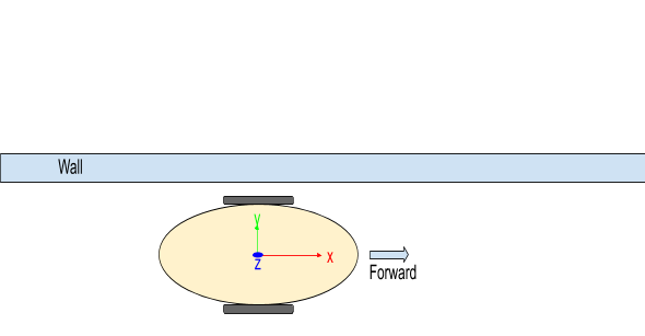
Wall Following

No matter how straight we drive, there will always be a little drift. Driving in a maze, this may cause our mouse to hit a wall. Using the ToF sensors on our mouse, we can use the distance to the wall as a reference to keep our mouse driving straight relative to the walls. For this section, you'll be implementing a P controller to perform wall following. Since our sensors have limitations, it doesn't need to correct for large angular errors, only smaller ones.

As you discuss how to implement this wall following controller remember that the controller needs an input, setpoint, and changeable value. How can our controller affect the angle the mouse is traveling? Don't be afraid to ask for help!

Checkoff #4

• Explain what you’re using for input, setpoint, and controllable value.
• Walk through the code you wrote for this wall following controller.
• Demonstrate wall following with the wall either on the left or right of your mouse.